Introduction
The creation and appreciation of music has been a ubiquitous human activity since the dawn of history. During my time at CATNIP Lab, one of the questions we asked was how recurrent neural networks may be able to gain an understanding of music. Originally, we wanted to use this as a bridge to generate hypotheses about how the brain processes music. Initially, I was training linear models and vanilla RNNs so that we would have the best hope of interpretting the computational processes which they learned; the old source code may be found at this repo. Eventually, I added to the framework some more state-of-the-art architectures (LSTMs and GRUs) as well as limit cycle initialization, I also cleaned up the code in 2021 and made it friendly to anyone who wants to download the repo.
Training Procedure
There are four standard datasets of piano music which have been used to benchmark recurrent neural networks in the past: JSB_Chorales (JSB standing for Johanne Sebastian Bach), Nottingham, MuseData, and Piano_midi. These datasets were used, for example, in this 2012 Bengio paper about RNN-RBMs. I initially wanted to incorporate RBMs or some other stochastic method into the readout, but was told by my colleagues that RBMs take too long to train.
The first step of training neural networks on this data is converting each song into 88 binary sequences. Each of the 88 sequences will correspond to 1 note, and each entry in the sequence will specify whether the note was on or off during that specific beat. Suppose a song is given by the binary sequences $y_{i,t}$, where $i$ specifies the note and $t$ secifies the time, or beat. The goal of our algorithm, is to take $y_{i,0..t-1}$ as input and then output a sequence $p_{i,t}$, specifying the probability that note $i$ is played at beat $t$. We can say the sequence of probabilities $p_{i,t}$ solves the task if it minimizes the cross entropy loss:
$$L(p, y)=-\sum_t\sum_i y_{i,t}\log(p_{i,t})$$
This is a classic loss function in machine learning, and essentially represents how surprised one expects to be about the event $y_{i,t}$ assuming its probability is $p_{i,t}$. The basic procedure is to use gradient descent to train a recurrent neural network to output a suitable $p_{i,t}$ given $y_{i,t}$. I empirically found that the RMSprop optimizer significantly outperforms both SGD and Adam for this task. I also implemented gradient clipping and orthogonal initialization in my framework, but found them to be unnecessary for improving performance. Initializing the $\tanh$ RNNs and GRUs to be near a direct sum of Hopf bifurcations (each 2D plane in the hidden state space is between a limit cycle and attracting fixed point) does improve performance. Unfortunately, these results will probably not be published because they still do not outperform RNN-RBMs.
Limit Cycle Intitialization
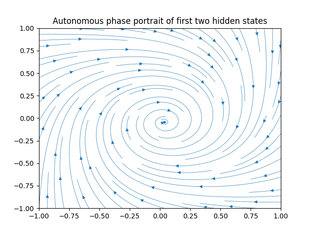
Much of my research at CATNIP Laboratory was on the treatment of recurrent neural networks as ordinary differentialy equations: Neural ODEs or NODEs. One mathematical observation which we made is that if one has an ODE with a 2D state-space and a limit cycle, the dynamics of its adjoint are stable in the sense that they also possess a limit cycle (see my figure below). This observation is important because the adjoint dynamics are the continuous analogue of backpropagating gradients; the result suggests that the backpropagating gradients of a limit cycle neural network cannot explode.
The idea of limit cycle initialization in my CyberBach project is that a $\tanh$ or GRU network with an even number of hidden units may be initialized so that each consecutive pair of hidden units has dynamics which look similar to what is pictured above. Of course, this only guarantees gradient stability at the first step, but I have had no trouble with exploding gradients using this initialization, and I think each limit cycle will indirectly act as a memory unit for the rest of the network.
The critical question, of course, is how we get a $\tanh$ or GRU network to exhibit a limit cycle. The intuition in 2D is not so hard: both systems are globally contracting their hidden state space to the region $[-1,1]^2$. Additionally, both systems are linearizeable around the origin. If we use a typical rotation matrix for the weights then we would expect the origin to be a stable spiral fixed point. However, if we scale that rotation matrix up enough then the origin can become a repelling spiral, meaning there will be a limit cycle in between.
Here I used WebGL to create a visualization of the $\tanh$ system:
Angle = 1
Scale = 1.5
This visualization plots a single trajectory in black and uses a popular technique called domain coloring for the rest of the vector field (specifically: red is an upperward pointing vector, green is to the lower right, and blue is to the lower left). It is quick and easy to render the phase portrait of the system like this. The vector field is given by:
$$F(x)=\tanh(Wx)-x$$
where $\tanh$ is applied to the vector $x$ element-wise and
$$W=\begin{bmatrix} S\cos(\theta) & -S\sin(\theta) \\ S\sin(\theta) & S\cos(\theta)\end{bmatrix}$$
is the weight matrix with angle $\theta$ and scale $S$. The Euler approximation of this vector field with step-size $1$ corresponds to a $\tanh$ recurrent neural network (without input, in these equations). This observation is what gave rise to the concept of Neural Ordinary Differential Equations.
As one can see from the interactive phase portrait, with any angle between about $0.2$ and $1.2$, and any scale slightly larger than $1$, the systems dynamics are given by a stable limit cycle. That is how the initialization works for the $\tanh$ networks: simply set the biases equal to zero and the requrrent weights equal to sequence of block diagonal $2\times2$ scaled rotation matrices with angle sampled between $0.2$ and $1.2$ and scale sampled between $1$ and $1.1$. Empirically, I found that a larger scaled will worsen performance greatly. My hypothesis is that the network prefers to be on the bifurcation point because with a limit cycle that is very structurally stable it will always have information from arbitrarily far back in the past resurfacing and acting as noise. That is, memory is good, but if you remember everything and your gradients are too stable you will not be able to distinguish relevant from irrelevant features. The GRU initialization works similarly, but one must also set all hidden weights except $n$-to-$h$ weights to $0$, and then double the scale of the rotation matrices (it is straightforward to work this out with some algebra on the GRU equations).
Music Synthesis
Now for the fun part. It is fairly straightforward to get neural networks trained to predict music to generate new music. Imagine as before we have the target song $y_{i,t}$, then we can ask the network to give probabilities of which notes will be played after the song has ended $p_{i, T+1}$. Then we can create a new binary sequence $q_{i, T+1}$ which is $1$ either for the notes which were given a probability greater than $0.5$, or the top 10 most probable notes (if the network tried to play more than 10 notes at a time it would sound very strange).
We can append $q_{i,T+1}$ to the end of $y_{i,t}$ and then feed it back to the network to get $p_{i,T+2}$, and $q_{i,T+2}$, and so on. For the synthesis procedure I also added some small Gaussian white noise to the input to try to make sure the network does not get locked into boring, highly periodic tunes.
The results of this experiment vary from aesthetic in a very bizarre way to extremely annoying. In the table below, I compared the output of 5 different models on one input from each of the 4 datasets. Each of the models is in the repo, and each of them was pre-trained on the JSB_Chorales dataset. Therefore, the output is not as diverse as it could be, and I encourage you to use my framework to train even more models and produce more strange tunes!
| Dataset | Original | TANH | Limit Cycle TANH | GRU | Limit Cycle GRU | LSTM |
|---|---|---|---|---|---|---|
| JSB_Chorales | ||||||
| Nottingham | ||||||
| MuseData | ||||||
| Piano_midi |