The Geometry of Zipf's Law

Jump to:
Introduction
Hilbert Spaces
The Laplace Operator
Kernels
Green's Theorem
Weyl's Law
Tying it All Together
Conclusions and Outlook

Introduction

Zipf's law is a seemingly mysterious phenomenon which has its origins in linguistics, but which is now known to arise in disparate domains including sociology, geology, genomics, physics, and even neuroscience. To state the law as it was originally observed for languages, let $f_n$ be the frequency (or total number of occurrences) of the nth most common word for some language. Then we have the following approximate equation:
$$f_n=\frac{f_1}{n}$$
Or, taking the logarithm for a more convenient form:
$$\log(f_n)=-\log(n)+\log(f_1)$$
For example, the most common word in English is "the," the second most common word is "be," and the third most common word is "to." If this law holds, we would expect "be" to occur 1/2 as often as "the," and "to" to occur 1/3 as often as "the."

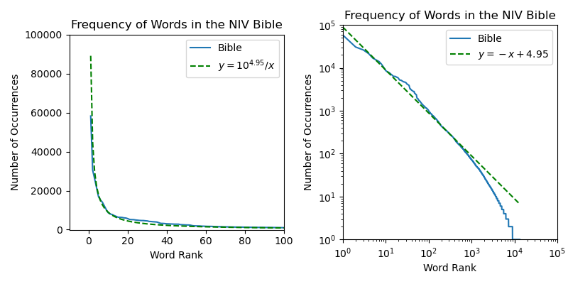
In reality, this is not exactly the case. Zipf's law only becomes accurate asymptotically, meaning the equations are only really accurate if $n$ is large. To demonstrate this, I performed the analysis on the NIV Bible and plotted my results below.

To represent the phenomenon in a very straightforward way, I have plotted on the left a curve proportional to $\frac{1}{x}$ as a green dotted line, and shown that it aligns roughly with the frequency of each word with respect to its rank. However, this way of plotting a power-law phenonenon is very limited, as it shows us only a few orders magnitude. The more common way to plot this is shown on the right, where the logarithm of the number of occurrences is plotted with respect to the logarithm of the rank of each word. Transformed to these coordinates, the data nearly follows a straight line for 3 orders of magnitude!

You can find my code, which includes preprocessing a PDF and cleaning the data, here. In my analysis, plural and non-plural words were considered as the same. However, different conjugations of the same verb are not identified. I would wager you could get an even better fit to a straight line if you considered linguistic artifacts like this.

Something which probably stands out at this point is that the many authors of the Bible most probably had no idea about exponents, logarithms, lines of best fit, or even equations. Indeed, this distribution of words is something that arose completely naturally, and it has been observed across many different corpuses of text in many different languages. Not only that, this distribution has been observed in the the noise spectrum of electrical circuits, Earthquake magnitudes, the sizes of cities, and even the frequency of amino acid sequences in the Zebra fish.

Although the ubiquity of this distribution may be initially surprising, each paper which I linked constains its own explanation for the phenomenon. However, the explanation which I want to dive into with this article comes from computational neuroscience, and may even have deep consequences for machine learning. The main paper which I'll be referring to is Stringer and Pachitariu et al.. The main body of this paper shows empirically that the visual cortex of the mouse is exhibiting Zipf's in a way which I'll elaborate on later in the article. Contained in the supplement of the paper is a very elegant and insightful proof for why we actually expect this distribution to emerge.

In order to understand the reasoning of Stringer and Pachitariu, we are going to have to introduce some linear algebra before delving into differential geometry, generalizing the Fourier transform, and tying it all back to the nature of representation itself, so buckle up and get ready for some spicy math!

Hilbert Spaces

For the rest of this article, I will invite you to think of functions as vectors. For some readers this might be familiar, but for those who are new to the concept remember that for any $f,g:\mathbb{R}\rightarrow\mathbb{R}$ we still have that, for all scalars $c\in\mathbb{R}$, $f(x)+cg(x)$ is still a function $\mathbb{R}\rightarrow\mathbb{R}$. We will use the notation $\mathcal{C}(S,\mathbb{R})$ to denote the vector space of continuous functions from $S$ to $\mathbb{R}$. For example $S$ could be the natural numbers $\mathbb{N}$, an interval $[0,1]$, a square $[0,1]\times [0,1]$, or a more complicated space.

An extremely important subspace of $\mathcal{C}(\mathbb{R},\mathbb{R})$ is $L^2(\mathbb{R})$. This subspace is defined such that for all $f\in L^2(\mathbb{R})$, we have that the quantitity
$$\langle f,f \rangle =\int_{-\infty}^{\infty}|f(x)|^2dx$$
is well defined. For general $f,g\in L^2(\mathbb{R})$, we define
$$\langle f,g \rangle =\int_{-\infty}^{\infty}f(x)g(x)dx$$
The operation $\langle\cdot,\cdot\rangle$ is referred to as the inner product on this space. A vector space supporting such an operation is referred to as a Hilbert space (note for advanced readers: actually, the metric induced by the inner product must be complete for it to be defined as a Hilbert space).

To see the intuition for this definition: we might want to think of the value $f(x)$ as the entry of the vector at index $x$. We might also want to (very intuitively) think of the integral sign $\int$ as if it were summation $\sum$. In that case, the operation defined above is precisely the infinite-dimensional generalization of the dot product. This is even more clear to see if we think of $L^2(\mathbb{N})$, where the equivalent of integration is again summation, so we have that for sequences $a,b\in L^2(\mathbb{N})$ the inner product is defined as:
$$\langle a,b \rangle =\sum_{i=0}^{\infty}a_i b_i$$ which is simply the dot product with infinitely many indices!

The Laplace Operator

Let's assume from now on that our domain space $S$ is compact, meaning it doesn't go on forever. $S$ could be a circle, sphere, line segment, or rectangle, for example. We will also assume that all of our functions are zero on the boundary, if a boundary exists. Note that the functions still form a vector space with this restriction.

One of the most important linear operators which we can define on $L^2(S)$ is the Laplace operator $\Delta$. If $S$ is an interval, $[0,a]$, then we have the following definition:
$$\Delta=-\frac{d}{dx^2}$$
That is, $\Delta$ is simply the second derivative operator. In this case, $\Delta$ measures the concavity, of its input function: how much the function is curving up or down. In the same way we can define an eigenvector equation in a finite-dimensional space, we can define an eigenfunction equation for an operator on an infinite-dimensional space:
$$\Delta v_{\lambda}=\lambda v_{\lambda}$$
In words, this equation is saying that the concavity of $v_{\lambda}(x)$ at $x$ is proportional to $x$ for all $x$. The $\sin$ function is the solution to this equation:
$$v_{\lambda}(x)=\sqrt{\frac{2}{a}}\sin\big(\sqrt{\lambda}x\big)$$
Since we are enforcing the condition that $v_{\lambda}$ is $0$ both at $x=0$ and $x=a$, we must have that all eigenvalues are of the form $\lambda=\sqrt{\frac{\pi^2 n^2}{a}}$, where $n$ is an integer. $\sqrt{\frac{2}{a}}$ is normalizing factor such that the norm of each function is $1$ (you can check this by computing the integral of the eigenfunction squared).

An essential result which we will be using is that the eigenfunctions $v_{\lambda}$ form an orthonormal basis for the entire vector space $L^2([0,a])$!

In order to prove orthonormality, you can simply compute the integrals $\int v_{\lambda}(x)v_{\mu}(x)dx$. When $\lambda=\mu$, you should find that the integral evaluates to $1$, otherwise you should find that its value is $0$.

When we say $\{v_{\lambda}\}$ is a basis for $L^2([0,a])$, we mean that for any function $f\in L^2([0,a])$ there are coefficients $c_{\lambda}$ (called the Foureir coefficients) for each eigenvalue $\lambda$, such that we have the following decomposition:
$$f(x)=\sum_{\lambda}c_{\lambda}v_{\lambda}(x)$$
In order to persuade you that the set of eigenfunctions also forms a basis for the space of all square-integrable function, I sketched below the functions $\sin(2\pi x)$, $\sin(6\pi x)$, and $\sin(18\pi x)$ on the interval $[0,1]$ in the first 3 panels. In the fourth panel, I sketched a sum:
$$A\sin(2\pi x) + B\sin(6\pi x) + C\sin(18\pi x)$$
where the coefficients $A$, $B$, and $C$ can be adjusted with the sliders!

The goal here is to illustrate that with only 3 basis functions, we can achieve a wide diversity of differently-shaped functions. The overarching idea is that the low-eigenvalue functions (i.e. $\sin(2\pi x)$) define the broad features of the function while the high-eigenvalue functions (i.e. $\sin(18\pi x)$) define the precise details of the function.

This decomposition is known as Fourier decomposition, and its fundametally about projecting square-integrable functions onto the orthonormal eigenbasis of $\Delta$

If we turn the interval into a prism, $[0,a]^N$, then $\Delta$ is a sum of second derivative operators:
$$\Delta=-\sum_{k=1}^N \frac{\partial^2}{\partial x^2_k}$$
Where each $\frac{\partial^2}{\partial x_k^2}$ is a second derivative with respect to the particular variable $x_k$. If we have the graph of a function $f(x_1,...,x_N)$ then its $N$ perpendicular cross sections with respect to the axes define $N$ curves, and $\Delta$ can be thought of as summing the concavities of those curves.

It turns out that the eigenfunctions of $\Delta$ form an orthonormal basis for $L^2(\mathbb{R}^2)$ as well! If our domain is $[0,1]\times[0,1]$ then, enforcing our boundary condition of zero, the eigenfunctions of $\Delta$ are given by:
$$v_{m,n}(x,y)=\sin(\pi m x)\sin(\pi n y)$$
Whose corresponding eigenvalue is given by $\pi^2(m^2+n^2)$.

To convince you in a similar manner that these functions do indeed form a basis, I've created a similar visualization. This time, however, I plot colors on the 2D plane with purple representing positive values of the function and green representing negative values. From left to right we have $\sin(\pi x)\sin(2\pi y)$, $\;\sin(3\pi x)\sin(5\pi y)$, $\;\sin(7\pi x)\sin(11\pi y)$, and finally their sum weighted again by $A$, $B$, and $C$.

If you tweak the sliders long enough, you will come up with a wide variety of configurations in the 4th panel. Just imagine what could be created with infinitely many basis functions!

It turns out that, whenever a space $M$ is Riemannian, meaning it has tangent spaces and a way to transport vectors between tangent spaces, it has a corresponding Laplace operator $\Delta_M$. Whenever the space is compact, meaning it doesn't go on forever, a countable set of eigenfunctions From $\Delta_M$ will form an orthonormal basis for $L^2(M)$. Examples of Riemannian spaces include $\mathbb{R}^n$ for any $n$, as well as many of its subsets such as the double torus, Klein bottle, or projective space, which we will unfortunately not visualize here.

If we are willing to except some hand-waving, it is reasonable to expect that the set of all images of natural scenes form a Riemannian space. Consider that all $100\times 100$ images exist in $\mathbb{R}^{100\times100\times 3}$, for $100\times 100$ pixels and 3 channels (red, green, blue) at each pixel. Most points in this space would look like chaotic nonsense to us, but the space of natural images (natural meaning photographed, not computer-generated) is "small" in some sense. For one thing, it is compact, because if it did go on forever the brightness or darkness of some pixel could go to infinity, which makes no real sense.

Although it may initially seem bizarre, it is a natural assumption to make in theoretical data science that a dataset sampled within Euclidean space has Riemannian geometry. We aren't going to delve into the intricacies of Riemannian geometry here, but we are going to demand that the space of natural images has some Laplace operator $\Delta$. The eigenfunctions of this operator are defined on the space of stimuli which Stringer and Pachitariu showed to the mouse. In order to understand how and why the neural activity of the mouse exhibits Zipf's law in response to the stimulus, we are going to relate the eigenvalues of this $\Delta$ operator to the response of the mouse brain.

Kernels

In the first section, we discussed what it means to have an inner product for functions. Now we should think about what it means to have a matrix product for functions. Suppose we have a function of two variables $K(x,y)$, we could think of $K$ as an infinite-dimensional matrix, with indices $x$ and $y$, in which case matrix multiplication of $f$ by $K$ would be defined as:
$$g(x)=\int K(x, y)f(y)dy$$
This is a very dangerous move: it requires that $K(x,\cdot)f(\cdot)$ is an integrable function for all $x$, so we can't just throw any old $K$ into this equation. However, if we are careful, the operation described above is called an integral operator and $K$ is referred to as its kernel.

Stringer and Pachitariu's theory rests on the assumption that their data of the mouse visual cortex record so many neurons (over ten thousand)= that the activity space can be thought of as infinite-dimensional. That is, we can choose a Hilbert space $\mathbb{H}$ for which $f\in\mathbb{H}$ represents the overall activity of the cortex and the domain of the function indexes the neurons. This means that $f(x)$ should be thought of as representing the activity of neuron $x$. Their experiments involved showing the mice videos and images, which should be primarily responsible for the variance in the activity of the neurons. Suppose we have a finite-dimensional Riemannian space $S$ with points $s\in S$ representing specific stimuli shown to the mouse. Then, assuming the brain has some degree of consistency, we automatically have a representation $\Phi:S\rightarrow \mathbb{H}$ which takes stimuli and returns cortex activity.

The central object required for developing a theory of how Zipf's law occurs in the brain is a kernel $K$ defined on the stimulus space $S$. The definition for $s,s'\in S$ is straightforward:
$$K(s,s')=\langle \Phi(s),\Phi(s') \rangle$$
To understand this definition, remember that the dot product of two finite-dimensional vectors $\langle u,v\rangle$ can be thought of as a product including their mangitudes and their similarity. This still applies in infinite dimensions: since we expect each stimulus to evoke a similar magnitude of activity, $K(s,s')=\langle\Phi(s),\Phi(s')\rangle$ can be thought of as the similarity of the responses $\Phi(s)$, $\Phi(s')$ of stimuli of $s$ and $s'$.

From now on, I will use $K$ to denote specifically this kernel for whatever representation $\Phi$ might be in question. In order to understand this definition, remember that our representation $\Phi$ takes a stimulus $s$ to a function describing neural activity. We can give a name to that function: $\Phi(s)=\phi(s,c)$ where $\phi(s,c)$ is now the activity of neuron $c$ given stimulus $s$.

In the same way a matrix has an eigenvector equation, a kernel $K$ has an eigenfunction equation:
$$\lambda v(s)=\int_{S}K(s,s')v(s')ds'$$
Where I used the notation $\int_{S}\cdot dS$ to denote integration over $S$.

Underlining the fact that $S$ is supposed to be a space representing natural images, $\mathbb{H}$ is the space of visual cortex activity, and $\Phi$ is the map taking an image and returning brain activity, what Stringer and Pachitariu found empirically is that the eigenvalues $\lambda_n$, in decreasing order, of the kernel $K$ (which can be computed from sampled data) have the following approximate relationship:
$$\lambda_n=\lambda_1 n^{-\alpha}$$
With $\alpha\simeq1$, this is exactly the same relationship appearing in Zipf's law! If you're anything like me, the fact that this distribution re-occurs in such an obscure setting is even more confusing than the original phenomenon itself. Before, we were just talking about the frequency of words, but now we're talking about the eigenvalues of some infinite-dimensional matrix? It turns out that the eigenvalues of $K$ can be related to the eigenvalues of $\Delta$ on $S$: the reason we see this decay pattern is because the brain must balance between the broad, abstract features analogous to the low-frequency eigenfunctions of $\Delta$, and the fine detailed features of the stimulus, encapsulated by the high-frequency eigenfunctions of $\Delta$. To see this in a more precise way, we will need two more theorems about the Laplace operator.

Green's Theorem

This is the simpler of the two theorems, and some version of this you will have learned in a calculus class. Consider the integral involving a single variable function $y(x)$:
$$\int_a^b \Big( \frac{dy}{dx} \Big)^2dx$$
By the product rule, we have
$$\int_a^b \Big( \frac{dy}{dx} \Big)^2dx=\int_a^b \frac{dy}{dx}\frac{dy}{dx}dx=y\frac{dy}{dx}\Bigg|_a^b-\int_a^b y\frac{d^2y}{dx^2}dx$$
In the second section we assumed boundary conditions of zero, meaning $y(a)=y(b)=0$, and we will do the same here. Bringing it all together we have
$$\int_a^b \Big( \frac{dy}{dx} \Big)^2dx=-\int_a^b y\frac{d^2y}{dx^2}\;dx$$
Remember that in one dimension, $\Delta=-\frac{d^2}{dx^2}$. In higher dimensions, our theorem generalizes nicely:
$$\int_S ( \nabla y )^2dx=\int_S y\Delta y dx$$
In this context we will refer to this equation as Green's theorem.

Weyl's Law

With this theorem, it will become a lot more clear why Zipf's law might emerge with the setup we have so far. When I first read its statement, it seemed simultaneously somewhat vague but also too convenient to be true. However, it turns out there is a very straightforward intuition for this theorem which can be turned into a proof for Euclidean spaces!

Suppose $M$ is a Riemannian space with dimension $d$ and Laplace operator $\Delta$. Denote by $N(\lambda)$ the number of eigenfunctions of $\Delta$ which have eigenvalue less than $\lambda$. Then there exists a constant $K$ such that
$$\lim_{\lambda\rightarrow\infty}\frac{N(\lambda)}{\lambda^{d/2}}=K$$
Which could also be written as $N(\lambda)=O(\lambda^{d/2})$, which could be said in English as "$N(\lambda)$ grows asymnptotically as fast as $\lambda^{d/2}$".

Although this may intially seem arcane, it is actually very clear when our space $M$ is an interval $[0,1]$ or a square $[0,1]\times[0,1]$. Starting with the interval $[0,1]$, recall that the eigenfunctions are given by $\sin(\pi nx)$, which I will plot below:

Let's think about what $N(\lambda)$ would be in this 1-dimensional case. If we have an eigenfunction with eigenvalue $\lambda'<\lambda$, then just by subsitution we have $\pi^2 n^2< \lambda$, which immediately tells us that $|\pi n|<\sqrt{\lambda}$. Since $n$ can be any integer, we immediately see that $N(\lambda)=O(\sqrt{\lambda})$ in dimension 1!

In dimension 2, for the square $[0,1]\times[0,1]$, we have that the eigenfunctions are $\sin(\pi nx)\sin(\pi my)$. I'll plot these below in the same way as before:

In this case, we have that $\lambda=(m^2+n^2)\pi^2$, meaning $N(\lambda)$ counts all integer pairs $(n,m)$ such that $n^2+m^2\leq\frac{\lambda}{\pi^2}$. A simple way of thinking about this inequality is that it measures the number of integer grid points inside a disk of radius $\frac{\sqrt{\lambda}}{\pi}$. We know that as the disk grows larger, the number of grid points becomes closer and closer to its area, and since the area of the disk is proportional to the square radius, $\frac{\lambda}{\pi^2}$, this implies that $N(\lambda)$ is eventually approximately proportional to $\lambda$!

This very nice way to reason about Weyl's law generalizes to higher dimensions in a straightforward way. Suppose we have an $d$-cube specified by $d$ variables $x_k$ with $0\leq x_k\leq 1$. Then the eigenfunctions of $\Delta$, with our boundary conditions enforced will be specified by some integer frequency variables $n_1,n_2,\cdots,n_d$:
$$\prod_{i=1}^d \sin(n_i \pi x_i)$$
The eigenvalue of such a function will be $\pi^2\sum_i n_i^2$. Once again, the function $N(\lambda)$ will count the number of integer tuples $(n_1,n_2,\cdots,n_d)$ satisfying $n_1^2+n_2^2 + \cdots n_d^2\leq \frac{\lambda}{\pi^2}$. This inequality defines all integer grid-points within a $d$-ball of radius $\frac{\lambda^{1/2}}{\pi}$. The amount of $d$-space that a $d$-ball with radius $\frac{\lambda^{1/2}}{\pi}$ takes up is proportional to $\lambda^{d/2}$!

To recap: let's say $\textrm{Int}_d(r)$ is the number of integer grid points contained within a $d$-ball of radius $r$. Let's also define $\textrm{Vol}_d(r)$ to be the volume of a $d$-ball with radius $r$. If we accept that
$$\lim_{r\rightarrow\infty}\frac{\textrm{Int}_d(r)}{\textrm{Vol}_d(r)}=1$$
and that
$$\textrm{Vol}_d(r)=Ar^d$$
for some constant $A$, and we observe as above that for a Laplace operator on a $d$-cube,
$$N(\lambda)=\textrm{Int}_d\Big(\frac{\lambda^{1/2}}{\pi}\Big)$$
Putting this altogether suggest that this is indeed a constant $K$ such that
$$\lim_{\lambda\rightarrow\infty}\frac{N(\lambda)}{\lambda^{d/2}}=K$$
Every step of this proof sketch should be checked carefully, but in essence we have proven what we have set out to prove about the Laplace operator on a $d$-cube!

Our overall goal for this section is to show that Weyl's law holds for Riemannian spaces in general, which we have yet to do. The argument in the general case becomes much more difficult, so we will only think about it intuitively. Even for the most complicated Riemannian space, like a Klein bottle, triple torus, or the space of natural images, if we zoom in far enough we will see that the space locally looks like a square (or some higher dimensional cube). When we consider the very high frequency eigenfunctions on one of these spaces, on each square-like neighborhood they will actually look a lot like the eigenfunctions on the square, and the overall eigenfunction will look like a patchwork of these local eigenfunctions! Therefore, as the eigenvalues become asymptotically larger, the Euclidean argument becomes increasingly close to being correct, and the eigenvalue count $N(\lambda)$ goes asymptotically to $\lambda^{d/2}$!

You should retain some skepticism around this argument, but hopefully I've at least convinced you that Weyl's law is worth believing in, because now it's time to explain why we see Zipf's law in the brain.

Tying it All Together

Remember that our mathematical setup for explaining Stringer and Pachitariu's findings is that $S$ is a Riemannian space of dimension $d$ consisting of every image which is shown to the mouse, $\mathbb{H}$ is a Hilbert space representing the activity of every neuron in the mouse visual cortex, and a representation $\Phi:S\rightarrow\mathbb{H}$ defines the response of the brain to a given stimulus. What we are interested in is the covariance kernel $K(s,s')=\langle \Phi(s),\Phi(s')\rangle$ and we have found that its eigenvalues approximately follow the law $\lambda_n\propto n^{-1}$. Let's make two observations based on what an ideal mouse brain might use for the representation $\Phi$.

First of all, $\Phi(s)$ should retain as much information about the stimulus $s$ as possible. This means that if $s$ and $s'$ are different stimulus, $\Phi(s)$ and $\Phi(s')$ should be very different, meaning $K(s,s')$ should be near zero. In this case the kernel $K$ is almost like an infinite-dimensional diagonal matrix, and we can find its eigenvalues along the diagonal $K(s,s)$. Naturally, we expect $\Phi(s)$ and $\Phi(s')$ to have a similar magnitude (the brain's overall level of activity isn't changing that much), so $K(s,s)\simeq K(s',s')$, meaning we expect that $\lambda_n\simeq K$ for some constant $K$.

This is not the case, however, and the reason ultimately comes from a second observation. Let $\nabla$ be a derivative operator on the stimulus space. At a given stimulus $s$, $\nabla\Phi(s)$ gives a value in the Hilbert space $\mathbb{H}$ for how much the representation changes around $s$ due to some perturbation (for advanced readers: the argument does not depend on which vector field is used to assign perturbations to stimuli). Mice need to be able to recognize a visual stimulus regardless of small perturbations: a deadly snake with a missing scale is still a deadly snake, a family member with discolored fur is still a family member. Given an infinitesimal change in a stimulus, there should only be an infinitesimal change in representation. In mathematical terms, the expected derivative magnitude must be finite:
$$\int_S ||\nabla \Phi(s)||^2 dS<\infty$$
Starting from this assumption, we will show that if $\lambda_n$ are the eigenvalues of $K$ in decreasing order, we must have
$$\lim_{n\rightarrow\infty}\frac{\lambda_n}{n^{-1-2/d}}=0$$
Before we officially start, let's first define $v_i$ as the eigenfunction of $K$ with eigenvalue $\lambda_i$ and $w_i$ as the eigenfunction of $\Delta$ with eigenvalue $\eta_i$, and note that since both $\{v_i\}$ and $\{w_i\}$ are orthonormal bases we must have an infinite orthogonal matrix $A$ trasnforming one basis into the other, i.e. $v_i=\sum_j A_{ij} w_j$ and $w_i=\sum_j A_{ji} v_j$.

Second, note that since $\{v_i\}$ forms a basis of $L^2(S)$, we can write our representation as $\Phi(s)=\sum_i u_i v_i(s)$, where each $u_i\in\mathbb{H}$ can be computed simply by projecting $\Phi$ onto the eigenvector $v_i$:
$$u_i=\int_S \Phi(s) v_i(s) dS$$
This definition makes it easy to compute the inner product of $u_i$ with itself: $$\langle u_i,u_i\rangle = \int_{S\times S}\langle\Phi(s),\Phi(s')\rangle v_i(s)v_i(s')\; dS dS'=\int_{S\times S}K(s,s') v_i(s)v_i(s')\; dS dS'=\int_S \lambda_i v_i(s)\; dS=\lambda_i$$
These equalities follow from the definition of $u_i$, the definition of $K$, the definition of $\lambda_i$, and the fact that $v_i$ has norm 1, respectively.

Now we are ready to start toying with the expected magnitude of the derivative of $\Phi$. First, we will use the decomposition of $\Phi$ we just discovered:
$$\int_S ||\nabla\Phi||^2 \; dS=\int_S \sum_i ||u_i||^2||\nabla v_i||^2 \; dS=\int_S \sum_i \lambda_i||\nabla v_i||^2 \; dS$$
Now we get to use Green's theorem on each $v_i$ to transform the equation into a form which allows an analysis of the Laplace operator!
$$\int_S \sum_i \lambda_i ||\nabla v_i||^2 \; dS=\int_S \sum_i \lambda_i v_i \Delta v_i \; dS$$
Next, we will use our first observation about transforming the basis $\{v_i\}$ into the basis $\{w_i\}$:
$$\int_S \sum_i \lambda_i v_i \Delta v_i \; dS=\int_S \lambda_i \Bigg(\sum_j A_{ij}w_j\Bigg)\Delta \Bigg(\sum_k A_{ik}w_k\Bigg) \; dS$$
Rewriting the sum we obtain:
$$\int_S \lambda_i \Bigg(\sum_j A_{ij}w_j\Bigg)\Delta \Bigg(\sum_k A_{ik}w_k\Bigg) \; dS = \int_S \Bigg(\sum_{i,j,k}\lambda_i A_{ij}A_{jk} w_{j}\Delta w_k \Bigg)\; dS$$
Remember that, because theory are eigenfunctions of $\Delta$, $\Delta w_k =\eta_k w_k$! Also, the only two quantities in this integral which actually depend on a point $s$ in the stimulus space are the Laplace eigenfunctions $w_j$ and $w_k$, so we are allowed to bring the sum outside the integral:
$$\int_S \Bigg(\sum_{i,j,k}\lambda_i A_{ij}A_{jk} w_{j}\Delta w_k \Bigg)\; dS=\sum_{i,j,k}\lambda_i \eta_k A_{ij}A_{ik}\int_S w_j(s)w_k(s) dS$$
We can now apply the fact that $\{w_j\}$ is an orthonormal basis, $\int_S w_j(s)w_k(s)\;dS$ is $1$ if $j=k$ and $0$ otherwise. This means we can simply eliminate the $k$ index from our sum, and finally arrive at:
$$\int_S ||\nabla\Phi||^2 \; dS = \sum_{i,j}\lambda_i \eta_j A_{ij}^2$$
And now we see the fundamental relation from which our Zipfian distribution arose! Due to Weyl's law, as $j$ grows large $\eta_j$ grows like $j^{2/d}$. Therefore, $\lambda_i$ must shrink at least as fast $i^{-1-2/d}$ because $i^{-2/d}$ cancels the growth of $\eta_j$, and shrinking faster than $i^{-1}$ ensures that the series will not diverge because any series shrinking faster than $i^{-1}$ does not diverge.

Of course, this last paragraph is not a rigorous argument because $\lambda_i$ and $\eta_j$ are coupled through $A_{ij}$, which is probably not the identity matrix. Stringer and Pachitariu do make this into a rigorous argument in their supplemental material. Although the rigorous version is short, I will not reproduce it here because it is somewhat technical and would mainly distract from the spirit of the proof. If I've caught your attention so far, I really encourage you to read their paper.

Another thing you will probably be wondering is why the power law turns out to be $n^{-1-2/d}$ instead of $n^{-1}$ as promised. With the dataset of natural images which Stringer and Pachitariu showed to the mice, the intrinsic dimensionality of the data is very large, meaning $\frac{2}{d}\rightarrow 0$. Furthermore, remember our first observation: a representation which preservers a maximal amount of information will have a covariance eigenspectrum which is approximately constant, or flat. Our theorem shows that the decay of the eigenspectrum must be at least as fast as $n^{-1}$, so decaying barely faster indicates a balance between preserving information and preserving differentiability.

What Stringer and Pachitariu's experiments show is that, the mouse brain is preserving as much detail about what it sees as possible, while still retaining a representation which is stable to small perturbations! What's even more incredible about their paper is that they actually tried a set of experiments where the projected the images onto their first two principal axes, and found a decay of $n^{-2}$; projecting the images onto four axes showed a power law of $n^{-1.5}$, and eight axes showed a power law of approximately $n^{-1.25}$. The mouse brain is very robust! If this does not convince you to read the paper, I don't know what will.

Most of this section has been sketching a rigorous analytical proof of why we expect to see Zipf's law in the brain. I hope you found the argument as beautiful as I did! However, we have deviated somewhat from the intuitive geometrical spirit of this article. Thus, we need an example.

Suppose we uniformly sample a point $s$ on the circle, with its angle scaled to be within $[0,1)$. We can construct $\Phi(s)$ as a real-valued sequence like so:
$$\Phi_{2n-1}(s)=\frac{\cos(2\pi s)}{n^{\alpha/2}}\;\;\;\Phi_{2n}(s)=\frac{\sin(2\pi s)}{n^{\alpha/2}}$$
Where $\alpha>1$. First, check that $\Phi$ always produces a sequence whose squared elements form a convergent series. Then it can be checked that the covariance kernel of this representation has an eigenspectrum decaying as $n^{-\alpha}$. Intuitively, this function of a circle extracts every single frequency of the data sampled on the circle, and represents each one in inverse proportion to its frequency.

To understand the meaning of our theorem, let's look at a random projection of this map into 3 dimensions. Below, I've taken the first 300 components of $\Phi$ and projected them onto 3 completely random axes. You can zoom in and out with the mouse and adjust $\alpha$ with the slider.

The circle is a Riemannian space with dimension $d=1$. According to our theorem, we expect the derivative $\nabla \Phi$ to be finite whenever $\alpha\geq 1+\frac{2}{d}=3$. Although I can't illustrate it precisely since computers can only handle finitely many line segments, we can clearly see that when $\alpha>3$ we have a smoother curve and when $\alpha< 3$ we have a more fractal curve. That's because a fractal is fundamentally defined as an object which has non-trivial high-frequency structure, and a smooth object is defined as one which has trivial high-frequency structure. Adjusting $\alpha$ adjusts the weight given to higher frequencies.

What Stringer and Pachitariu have shown is that representations with a Zipf law, including the one found in the mouse brain, are perfectly on the boarder between smooth and fractal!

Conclusions and Outlook

I started this article by talking about the occurrences of words in text, and then I completely shifted gears to talk about the eigenspectrum of some kernel derived from neurological experiments. Is there any relation between these things? Zipf's law is the most common "hook" for people to start learning about general "power-law" phenomena, which are very ubiquitous and occur for a number of reasons. However, I do think that the explanation for Zipf's law in the brain can be tied back to the original Zipf's law.

Eigenfunctions of the covariance kernel can sort of be thought of as the atoms of the representation: they are all completely distinct from one another and the representation can be decomposed as a combination of them. Individual words in a language carry a very similar purpose. In this case, the "stimulus space" would actually be the space of human thought, which is, through the process of expresssion, mapped into the space of text in some language. The frequency of a certain word then corresponds to its "coefficient" in the decomposition, which would be analogous to the eigenvalue of a given eigenfunction.

This is a very hand-wavy explanation of the original Zipf's law. However, if we accept the analogy then we notice that Benoit Mandelbrot's idea, that Zipf's law emerges because language-users want to maximize the entropy of the language while keeping the energy consumption within reasonable bounds, appears a lot like Stringer and Pachitariu's argument!

Another interesting aspect of these findings is that the properties of the mouse brain's representation are very sought-after in machine learning. It often happens that, simply by adding imperceptible noise to an image of a car, we can cause a neural network to classify it as an image of a panda. This anomaly, known broadly as adversarial attacks, is caused by a large jump in the representation of the image despite only a very small perturbation to the input. If an artificial neural network were to use a power-law representation out-of-the-box, in the same way animals do, it would be almost completely free of adversarial attacks while still being able to extract all relevant features of the data!